All You Need To Know About Numpy

What Is NumPy?

NumPy stands for Numerical Python. It's the backbone of all kinds of scientific and numerical computing in Python. It vastly simplifies manipulating vectors and matrices.

Some of python’s leading packages relies on NumPy as a fundamental piece of their infrastructure (examples include pandas, scikit-learn, SciPy and TensorFlow).

In this post, we’ll look at some of the main ways to use NumPy and how it can represent different types of data before we can serve them to machine learning models.

Why NumPy?

You can do numerical calculations using pure Python. In the beginning, you might think Python is fast but once your data gets large, you'll start to notice slowdowns.

• The main reasons to use NumPy is because it's fast.

Woah, that's a huge difference there. Basically, the sum function using python is taking approx 17,000 microseconds whereas the sum using NumPy is taking just 55 microseconds. This time difference will have a huge impact on big projects.

Behind the scenes, the code in NumPy has been optimized to run using C which is much faster than Python.

• Apart from speed NumPy, arrays are more compact than Python lists. It uses much less memory to store data and it provides a mechanism of specifying the data types, which allows the code to be optimized even further.

• But, while a Python list can contain different data types within a single list, all of the elements in a NumPy array should have homogenous elements. The mathematical operations that are meant to be performed on arrays wouldn’t be possible if the arrays weren’t homogenous.

If your curious as to what causes this speed benefit, it's a process called vectorization. Vectorization aims to do calculations by avoiding loops as loops can create potential bottlenecks.

NumPy achieves vectorization through a process called broadcasting. We will look into it in more detail ahead.

Let's get started with NumPy.

Any time you want to use a package or library in your code, you first need to make it accessible.

In order to start using NumPy and all of the functions available in NumPy, you’ll need to import it. This can be easily done with this import statement:

import numpy as np

Datatype

The important thing to remember is that the main type in NumPy is ndarray, even though you might find different kinds of arrays but in the end, they all are ndarray.

ndarray is shorthand for the n-dimensional array.

Key Terms

• Array - A list of numbers, can be multi-dimensional.
• Scalar - A single number (e.g. 1).
• Vector - A list of numbers with 1-dimesion (e.g. np.array([1, 2, 3])).
• Matrix - A (usually) multi-dimensional list of numbers (e.g. np.array([[1, 2, 3], [4, 5, 6]])).

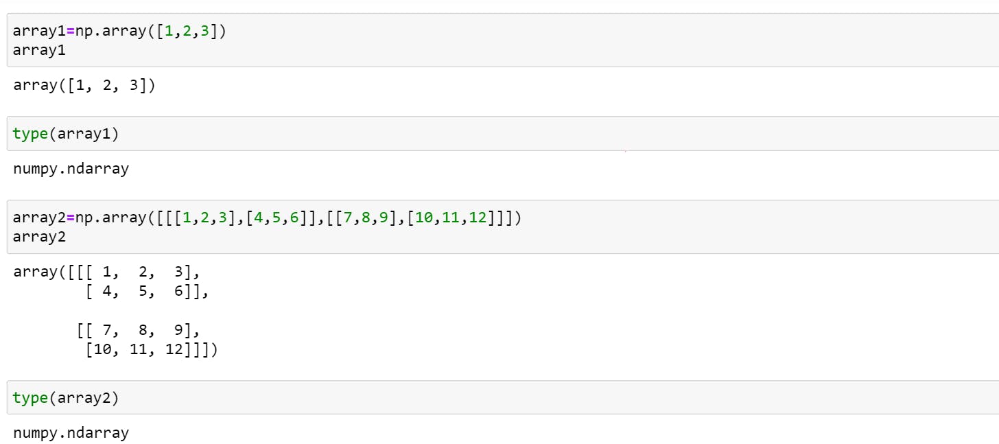By this, we can conclude that an operation you do on one array, will work on another.

Attributes

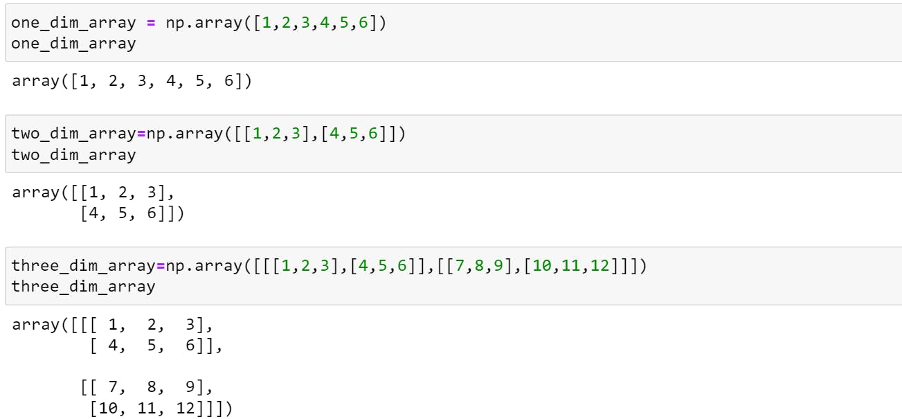
To understand all attributes and other methods let us define three arrays to get better understanding:

Code

Diagrammatically Explained

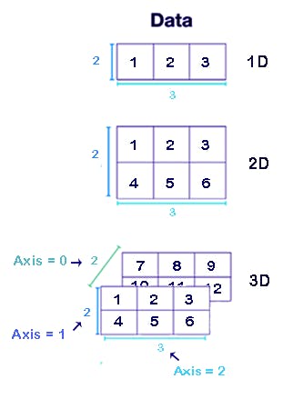
1. ndarray.ndim: It represents the number of dimensions (axes) of the ndarray.

   one_dim_array.ndim,two_dim_array.ndim,three_dim_array.ndim
   #Output=>(1, 2, 3)
   

2. ndarray.shape: Shape is a tuple of integers representing the size of the ndarray in each dimension.

   one_dim_array.shape,two_dim_array.shape,three_dim_array.shape
   #Output=>((6,), (2, 3), (2, 2, 3))
   

3. ndarray.size: Size is the total number of elements in the ndarray. In other words, it is the product of elements of shape.

   one_dim_array.size,two_dim_array.size,three_dim_array.size
   #Output=>(6, 6, 12)
   

4. ndarray.dtype: It shows the data type of the elements of a NumPy array.

   one_dim_array.dtype,two_dim_array.dtype,three_dim_array.dtype
   #Output=>int32 is the for all arrays
   

   Note: The size of the integer depends on the processor, so you may get a different answer from mine.

5. ndarray.itemsize: It returns the size (in bytes) of each element of a NumPy array. For example in below code, the item size is 4 because the array consists of integers (int32).

   one_dim_array.itemsize,two_dim_array.itemsize,three_dim_array.itemsize
   #Output=>(4, 4, 4)
   

   Note: 8 bits = 1 byte, so 32 bits = 4 bytes

6. ndarray.nbytes: It lists the total size (in bytes) of the array:

   one_dim_array.nbytes,two_dim_array.nbytes,three_dim_array.nbytes
   #Output=>(24, 24, 48)
   #24 = 4 bytes * 6 elements
   #24 = 4 bytes * 6 elements
   #48 = 4 bytes * 12 elements
   

   Creating Arrays

Apart from np.array method, you can also create arrays in many different ways.

1. np.zeros()

   np.zeros([1,4])
   #Output=>array([[0., 0.]])
   

2. np.ones()

   np.ones([1,4])
   #Output=>array([[1., 1., 1., 1.]])
   

3. np.arange()

   np.arange(2,12,4) 
   #np.arange(start,stop,step)
   #Output=>array([ 2,  6, 10])
   

4. np.linspace(): Creates an array with values that are spaced linearly in a specified interval

   np.linspace(0,10,6) 
   #np.linspace(start,stop, num_of_samples_to_generate)
   #Output=>array([ 0.,  2.,  4.,  6.,  8., 10.])
   

5. np.random.randint(): Returns random integers

   np.random.randint(2,10,3)  
   #np.random.randint(start,stop, num_of_samples_to_generate)
   #Output=>array([4, 4, 3])
   

Viewing arrays and matrices

Remember, because arrays and matrices are both ndarray's, they can be viewed in similar ways. Indexing in NumPy array starts with 0.

Let's check out our 3 arrays and diagram to understand better.

1. Array Indexing: It is very similar to list indexing.

2. Array Slicing: Just like you use square brackets to access individual array elements, you can also use them to access subarrays with the slice notation, marked by the colon (:) character.

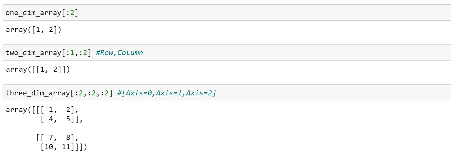
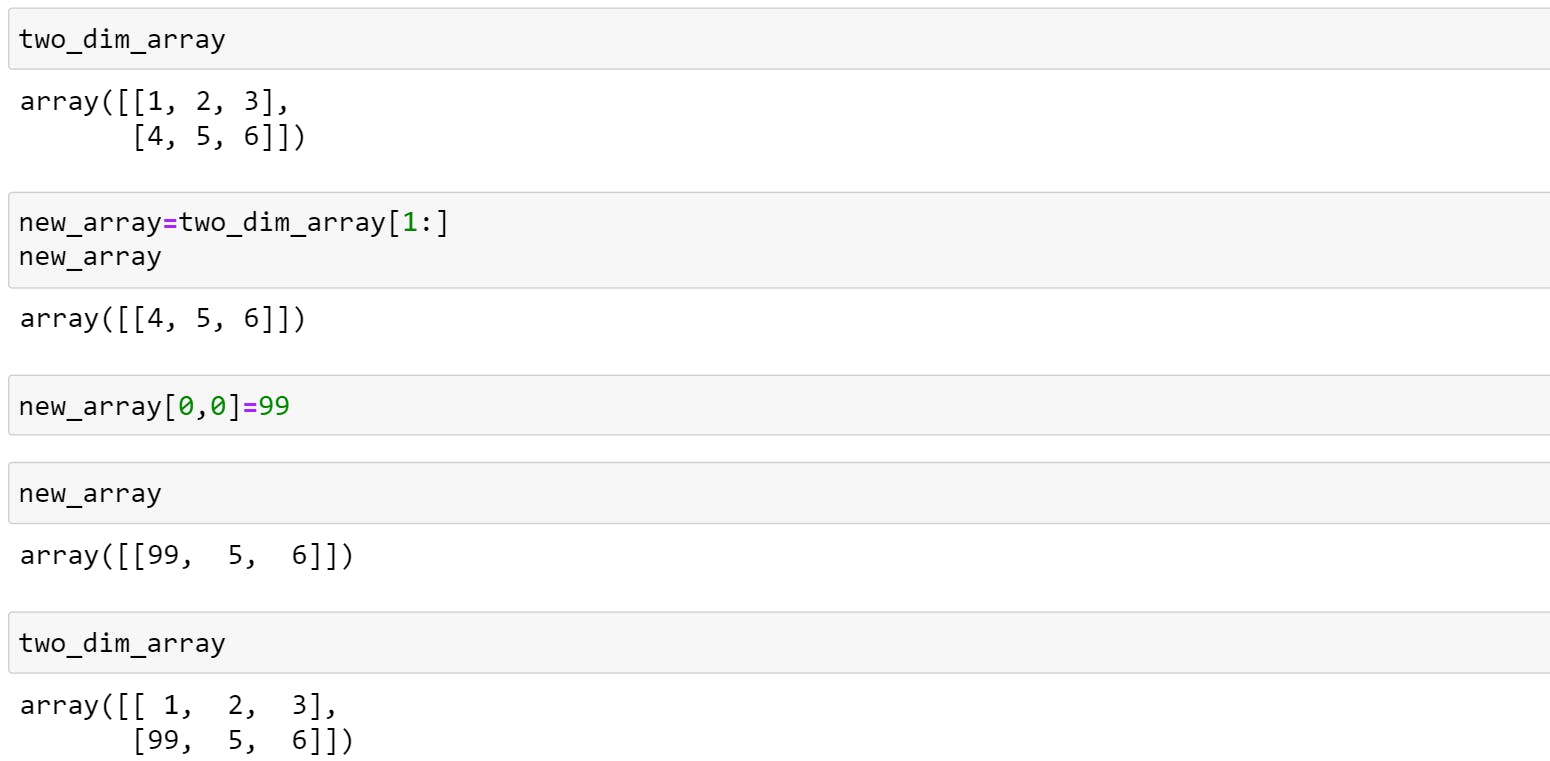
Note: One important thing to know in array slicing is that they return view rather than array data, so when you assign the sliced array to a new array and then change the value of the new array, it will affect the original one too.

This is a bit different from python list slicing. Let's look at an example to get a better understanding.

Manipulating & Comparing arrays

Arithmetic

• +, -, , /, //, *, %
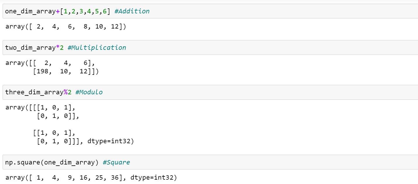
• np.exp()
• np.log()
• Dot product - np.dot()
• Broadcasting

Let's see few examples,

Simple Operations

Exponent and Logarithm

Let's add one dimension array and two dimension array to see their result.

Error, Uhmm.. What just happened?

operands could not be broadcast together with shapes (6,) (2,3)

This error occurred because when you operate on two arrays, NumPy compares their shapes element-wise. It starts with the trailing dimensions and works its way forward. Two dimensions are compatible when:

• they are equal, or
• one of them is 1

How to solve this?

Broadcasting

What Is Broadcasting?

The term broadcasting refers to the ability of NumPy to treat arrays of different shapes during arithmetic operations. Arithmetic operations on arrays are usually done on corresponding elements. If two arrays are of exactly the same shape, then these operations are smoothly performed.

We can use reshape method on either of the arrays to make it compatible. For example,

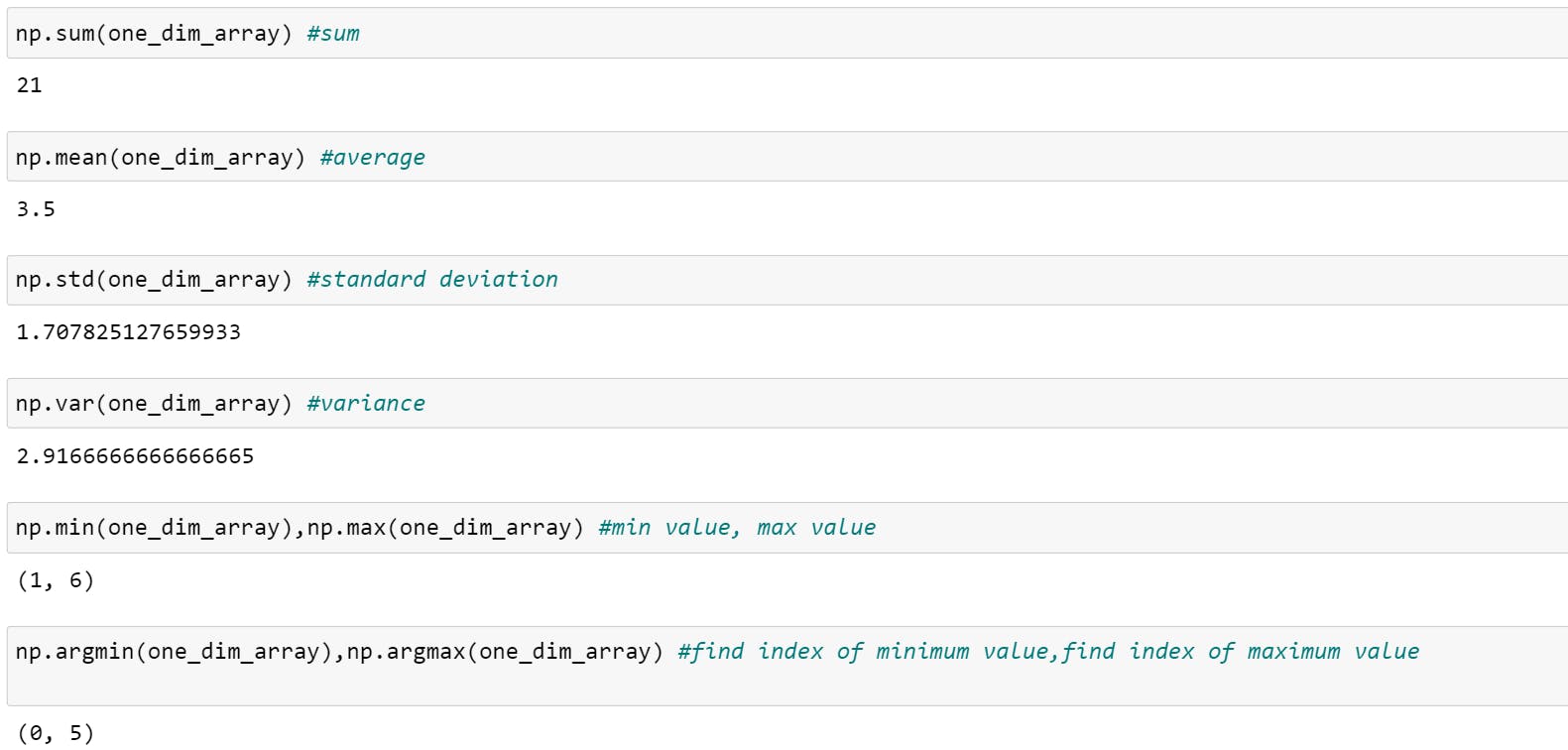
Aggregation

Aggregation

• np.sum()
• np.mean()
• np.std()
• np.var()
• np.min()
• np.max()
• np.argmin()
• np.argmax()

Transpose

The transpose of a matrix is an operator which flips a matrix over its diagonal; that is, it switches the row and column indices.

Dot Product

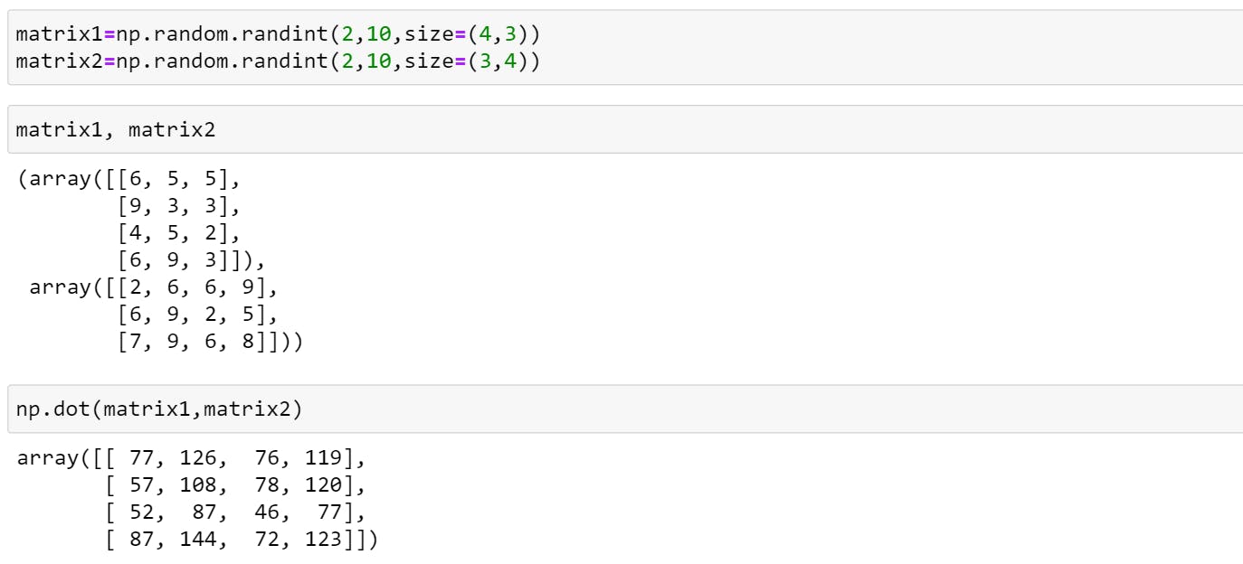
Dot products are done between the rows of the first matrix and the columns of the second matrix. Thus, the rows of the first matrix and columns of the second matrix must have the same length.

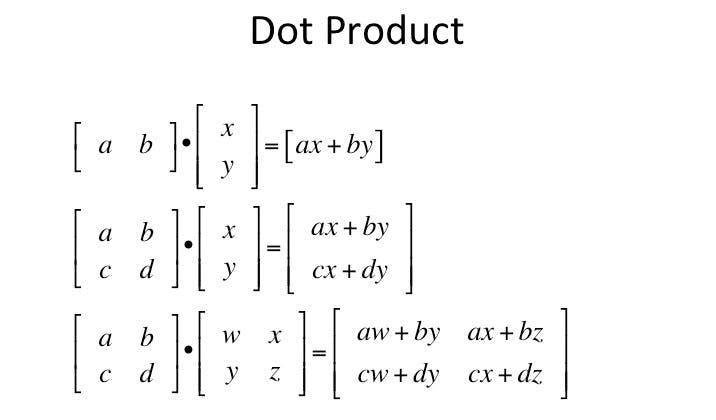
Let's see an example,

Comparison operators

Comparison operators include Less Than, Less Than or Equal to, Equal, Not Equal, Greater Than, and Greater Than or Equal to. An expression that compares two values and evaluates to True or False.

one_dim_array == two_dim_array
#Output=>False
one_dim_array > two_dim_array.reshape(6,)
#Output=>array([False, False, False, False, False, False])
one_dim_array <= two_dim_array.reshape(6,)
#Output=>array([ True,  True,  True,  True,  True,  True])

and so on...

Adding & Removing Data

Let's define one dimension array,

arr = np.array([1, 2, 3, 4, 5, 6, 7, 8])

Appened

You can add elements to your array with np.append() which takes two parameters array name and elements you want to add.

np.append(arr, [1,2.3,4])
#Output=>array([1, 2, 3, 4, 5, 6, 7, 8, 1, 2,3,4])

Delete

You can delete an element with np.delete().

np.delete(arr, 2)
#Output=>array([1, 3, 4, 5, 6, 7, 8, 1, 3, 4])

Array Concatenation and Splitting

Concatenation

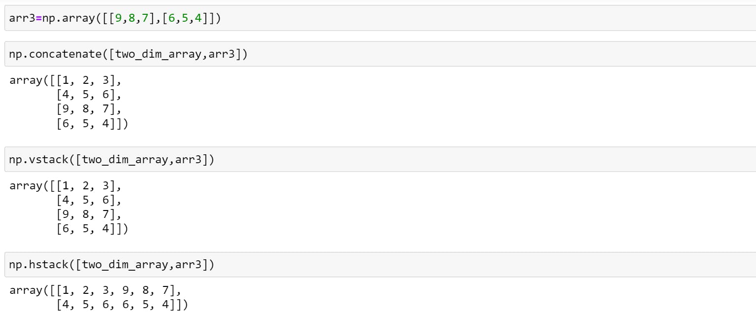
Concatenation (joining) of two arrays in NumPy, can be accomplished using the np.concatenate, np.vstack, and np.hstack.

For one dimension array:

It can also be used for two-dimensional arrays:

Spiliting Of Arrays

Splitting of arrays in NumPy, can be accomplished using the np.split, np.vsplit, and np.hsplit.

Note: Split an array into multiple sub-arrays of equal size.

If you don't want to split the array in equal size then you should mention integer in square brackets.

x = np.array([1,2,3,4,5,6,11,8,9])
np.hsplit(x,[8])
#Output=>[array([ 1,  2,  3,  4,  5,  6, 11,  8]), array([9])]

Sorting Array,

We have come to the last section of this article.

• np.sort()
• np.argsort()

Let's define new array with random numbers,

x = [4,9,55,34,12,3,67]

1. np.sort() : Returns the sorted array

   np.sort(x)
   #Output=>[3, 4, 9, 12, 34, 55, 67]
   

2. np.argsort(): Returns the indices that would sort an array

   np.argsort(x)
   #Output=>array([5, 0, 1, 4, 3, 2, 6]
   

   So, That's it for this article. I hope you learned something new. Please comment down if you find anything incorrect, or you want to share more information about the topic discussed above.